R Day Slides
R was created here
Not just statistics

Danielle Navarro - Stalk and Feather
Disclaimer
Our goal
NO = Learning statistics
Our goal
YES = Getting accustomed to R and grasping its use
NO = Learning statistics
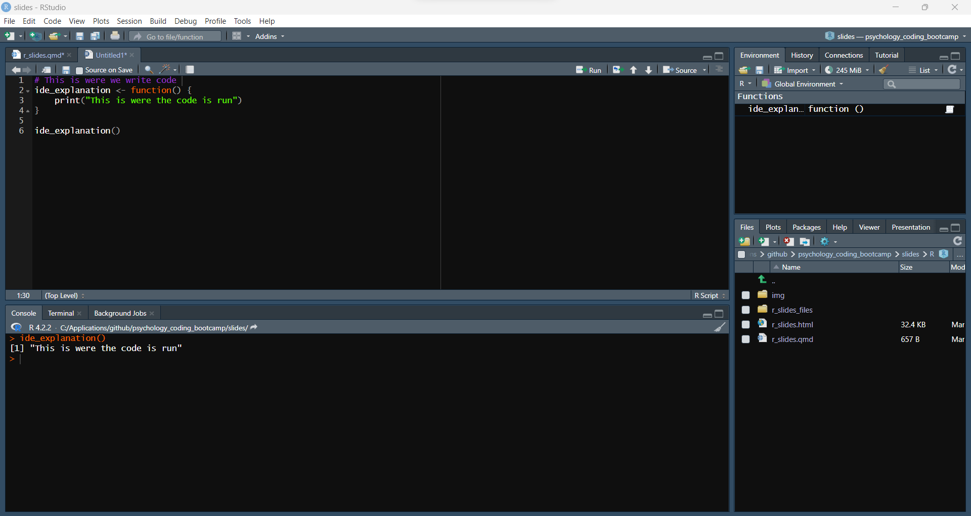
Rstudio
Rstudio (Posit)
Rstudio (Posit)
Rstudio (Posit)
Rstudio (Posit)
Rstudio (Posit)
Rmarkdown
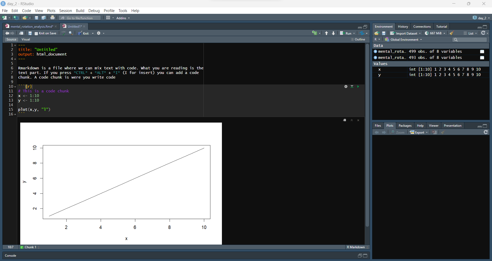
Rmarkdown
Rmarkdown
Today
Today
- R basics
- Loading and Cleaning data (
janitor,dplyr) - Pipe (
%>%) - Plotting with
ggplot - K-means clustering
Loading and cleaning data
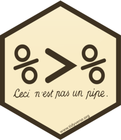
Pipe
Pipe
Let’s load, clean up names and select columns all in one go with the pipe (%>%)
Let’s load, clean up names and select columns all in one go with the pipe (%>%)
Let’s load, clean up names and select columns all in one go with the pipe (%>%)
Let’s load, clean up names and select columns all in one go with the pipe (%>%)
Filtering
Filtering
Filtering
Summarising
Summarising
Summarising
Summarising
Summarising
space_data <- space_data %>%
    group_by(movie) %>%
    summarise(frequency_space = sum(normalised_frequency)) %>%
    ungroup()
west_data <- west_data %>%
group_by(movie) %>%
summarise(frequency_west = sum(normalised_frequency)) %>
ungroup()
winter_data <- winter_data %>%
group_by(movie) %>%
summarise(frequency_winter = sum(normalised_frequency)) %>%
ungroup()Put all together
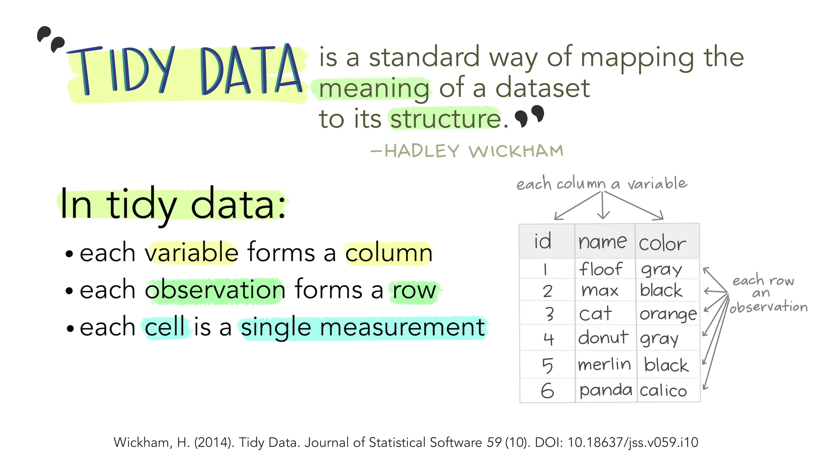
In R we usually want to work with data stored in one dataset
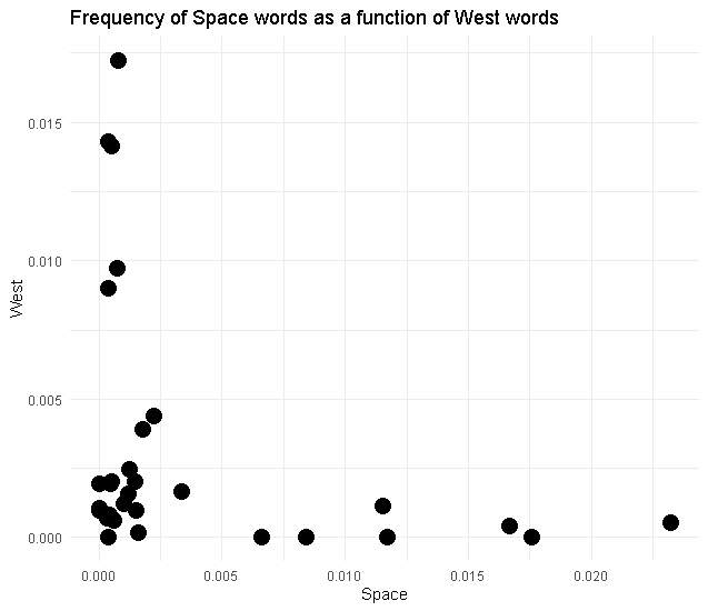
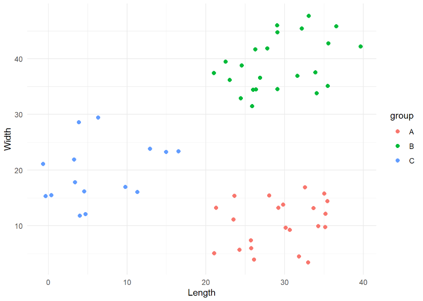
ggplot
We will make this
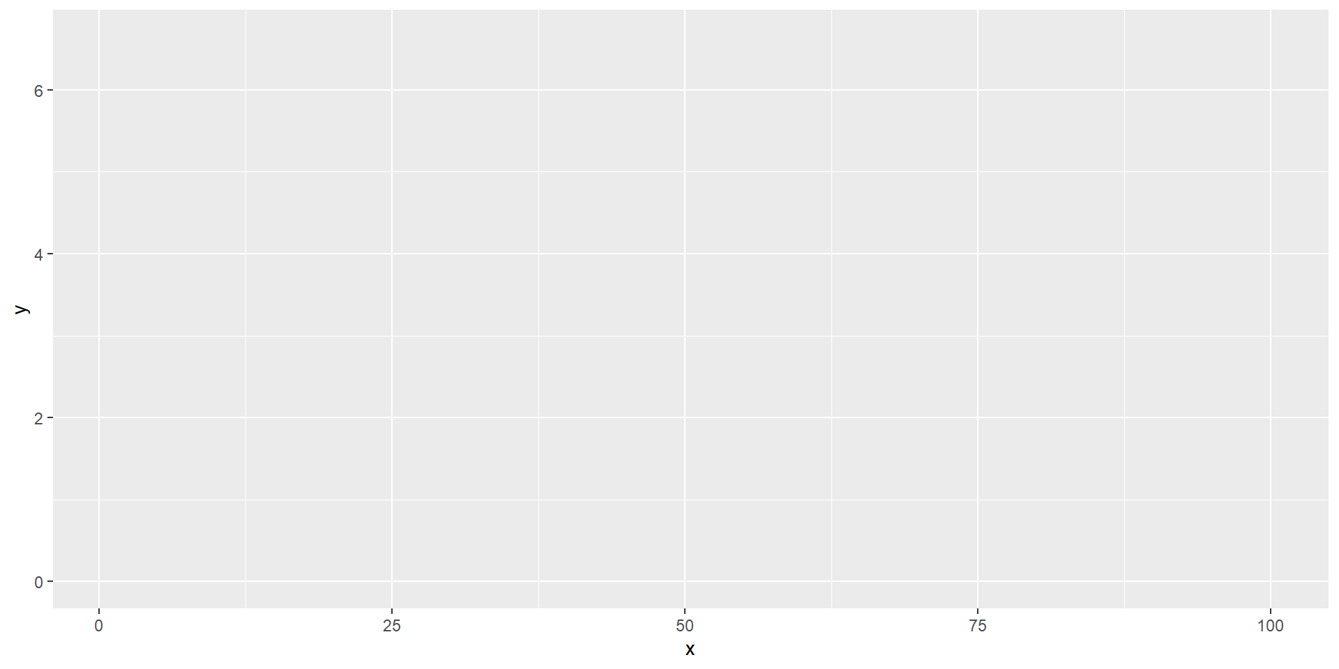
ggplot: coding a painting
Start with a blank canvas

ggplot: coding a painting
Add a primer - the x and y axis
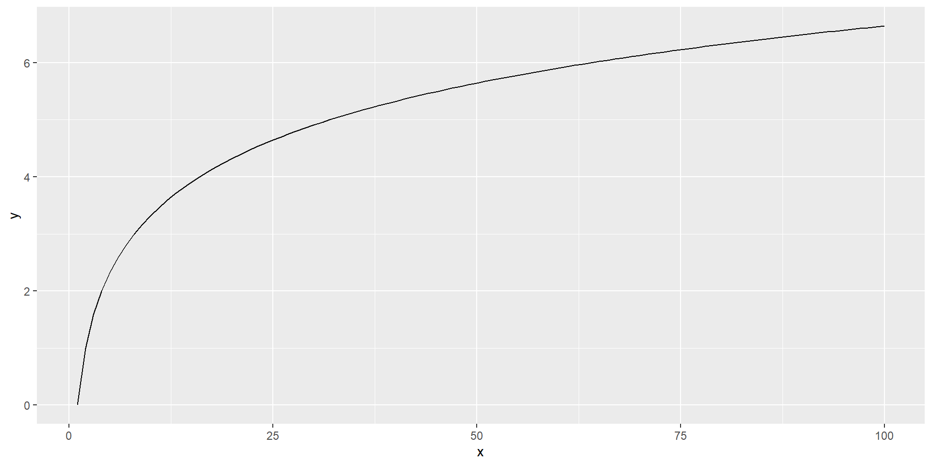
ggplot: coding a painting
Add the subject
ggplot: coding a painting
Make it stylish
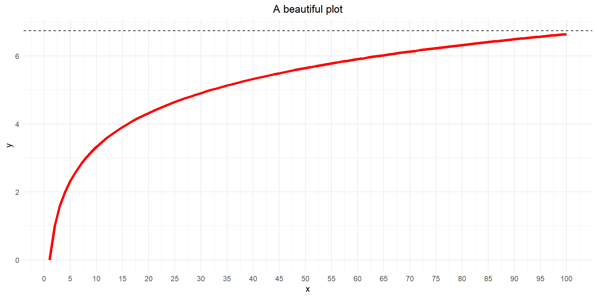
Our plot
Our plot
Our plot
Our plot
Layers
Layers stack on top of each other!
We can look at an example (if we have time)
| id | Q1 | Q2 | Q3 |
|---|---|---|---|
| 1 | 43.4947976 | -4.1284871 | 139.7134 |
| 2 | 0.5145435 | 5.1488069 | 134.8856 |
| 3 | 42.3330507 | -0.3975525 | 146.8220 |
| id | question | score |
|---|---|---|
| 1 | Q1 | 43.4947976 |
| 1 | Q2 | -4.1284871 |
| 1 | Q3 | 139.7134024 |
| 2 | Q1 | 0.5145435 |
| 2 | Q2 | 5.1488069 |
| 2 | Q3 | 134.8855685 |
| 3 | Q1 | 42.3330507 |
| 3 | Q2 | -0.3975525 |
| 3 | Q3 | 146.8220343 |
Long format rules (Einstein, 1905)
# Boxplots with scatterplot layer on top
box_with_scatter <- long_data %>%
    # Remove winter cause it's distribution ruins the visualisation here
    filter(category != 'frequency_winter') %>%
    # Set up canvas
    ggplot(aes(x = category, y = frequency)) +
    # First layer: boxplot
    geom_violin(aes(fill=category)) +
    # Second layer: scatterplot
    geom_point(position = position_jitter(width=0.1), size=4, alpha=.60 ) +
    # Title
    labs(title = 'Boxplot + Scatterplot') +
    # Change x labels
    scale_x_discrete(labels=c('space', 'west', 'winter')) +
    # Remove legend
    theme_minimal() +
    theme(legend.position = 'none')
# Boxplots with scatterplot layer on top
scatter_with_box <- long_data %>%
# Remove winter cause it's distribution ruins the visualisation here
filter(category != 'frequency_winter') %>%
# Set up canvas
ggplot(aes(x = category, y = frequency)) +
# First layer: scatterplot
geom_point(position = position_jitter(width=0.1), size=4, alpha=.60 ) +
# Second layer: boxplot
geom_boxplot(aes(fill=category)) +
# Title
labs(title = 'Scatterplot + Boxplot') +
# Change x labels
scale_x_discrete(labels=c('space', 'west', 'winter')) +
# Remove legend
theme_minimal() +
theme(legend.position = 'none')kmeans
kmeans
kmeans
kmeans
kmeans
kmeans
kmeans
k. (2023, April 13). In Wikipedia. https://en.wikipedia.org/wiki/K-means_clustering
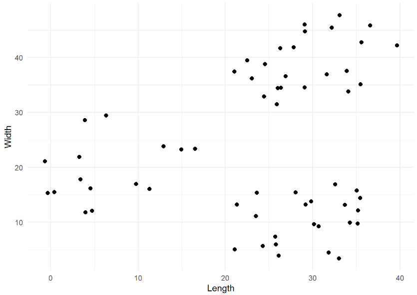
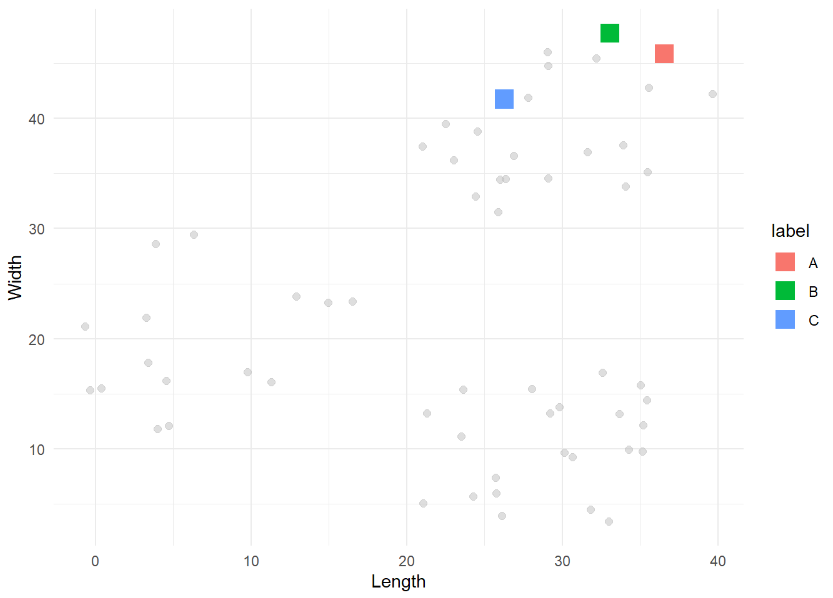
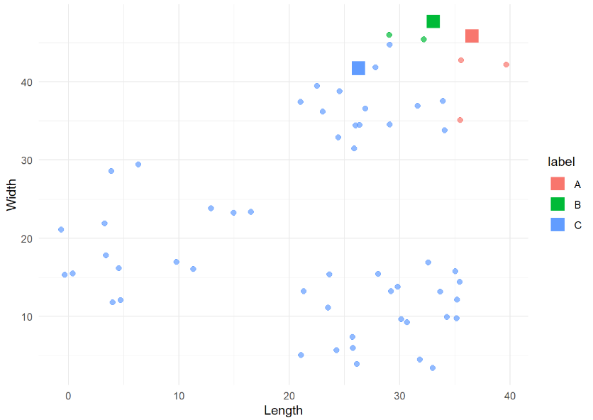
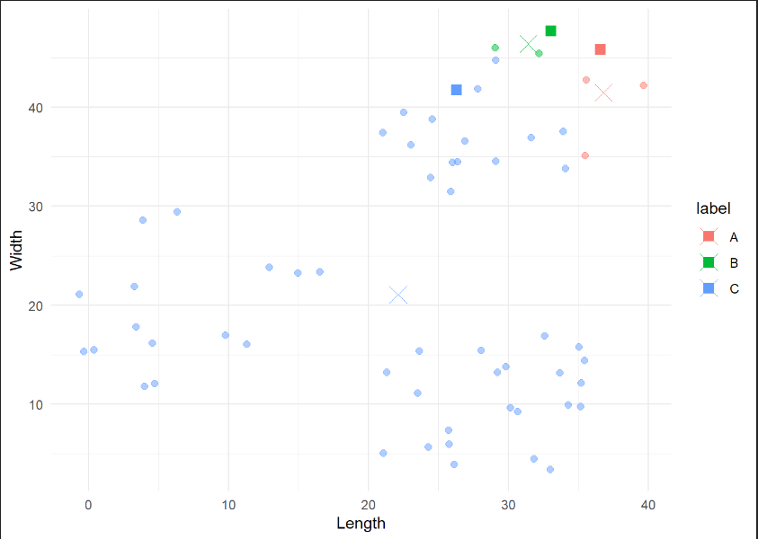
Kmeans Example
EEG data segmentation (microstates)
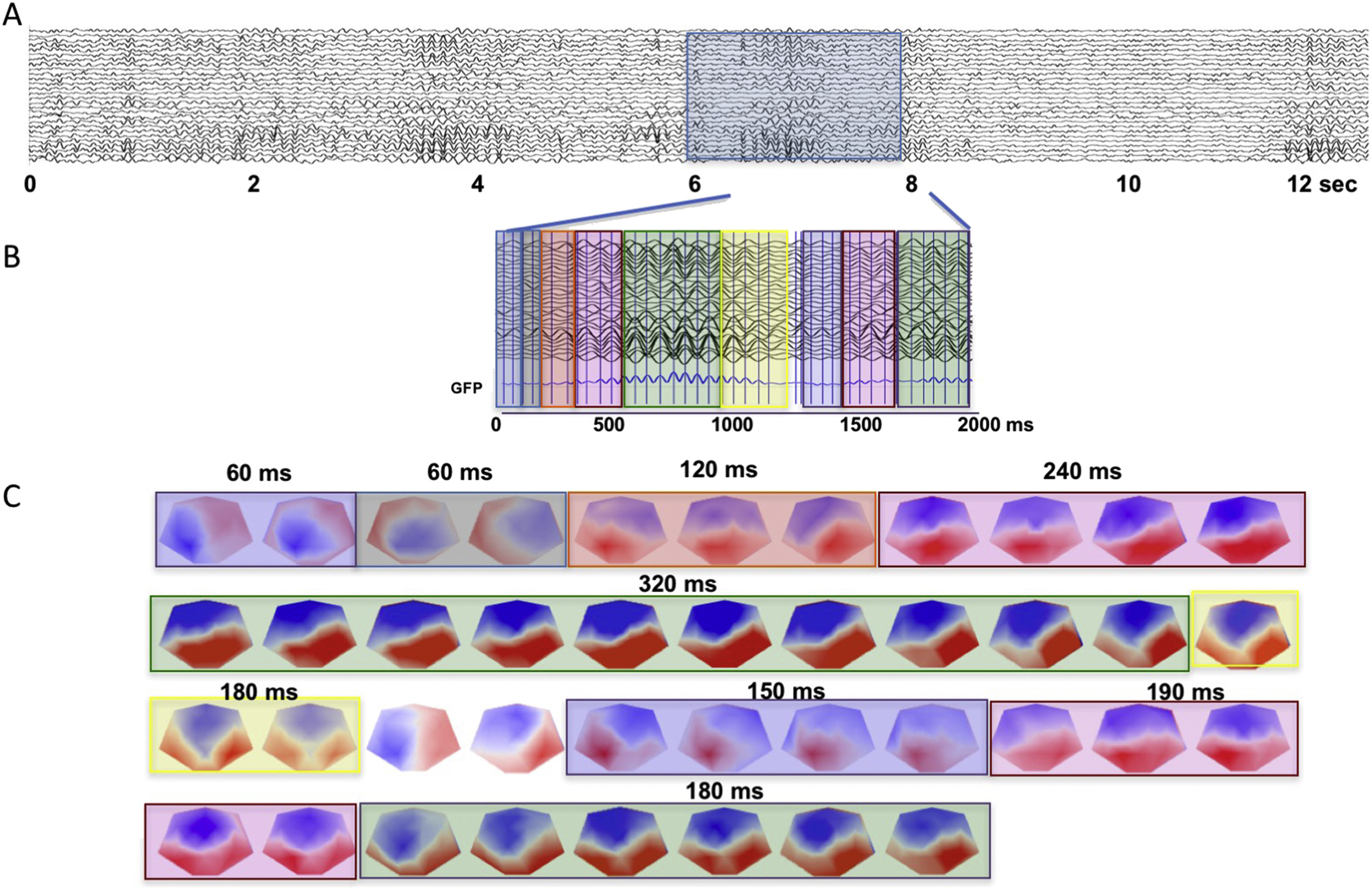
Michel, C. M., & Koenig, T. (2018). EEG microstates as a tool for studying the temporal dynamics of whole-brain neuronal networks: A review. NeuroImage, 180(Pt B), 577–593. https://doi.org/10.1016/j.neuroimage.2017.11.062
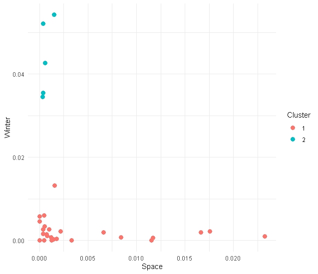
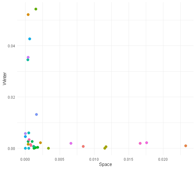
kmeans 2D
We start by considering only 2 dimensions of our data (Space & Winter)
# kmeans model on two dimensions
km_model_space_winter <- kmeans(category_data[, c('frequency_space', 'frequency_winter')], centers = 2)

# Add cluster info to data
cluster_results <- cbind(category_data, "cluster"= km_model$cluster)

# Plot the result
cluster_results %>%
    ggplot(aes(x = frequency_space, y = frequency_winter, colour = as.factor(cluster))) +
    geom_point(size=3) +
    labs(x = 'Space',
         y = 'Winter',
         colour = 'Cluster') +
    theme_minimal()
You should see something like this (possibly different though!)
Go beyond 2 Dimensions
In this data set we have three features to feed our kmeans (space, west and winter). Let’s use them all!
Go beyond 2 Dimensions
Go beyond 2 Dimensions
Go beyond 2 Dimensions
Go beyond 2 Dimensions
This is not essential (3D plotting in R is annoying/tricky)
Go beyond 2 Dimensions
This is not essential (3D plotting in R is tricky)
How many clusters
How many clusters
How many clusters
How many clusters
?
How many clusters
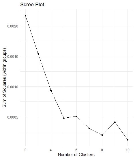
A simple way is to try to maximise the “homogeneity” within each group. We can operationalise “homogeneity” through the Sum of Squares.
How many clusters
But… we don’t want to overfit the data
Let’s iterate
iterative_kmeans <- function(in_data, k_max) {

    # Create a vector to store the within-cluster sum of squares for each iteration
    within_sum_squares <- c()

    # Repeat the clustering changing systematically the number of clusters
    for (iCluster in 2:k_max) {
        # Compute k-means
        current_km_model <- kmeans(in_data, centers = iCluster)
        # Extract within-cluster sum of squares
        within_sum_squares <- append(within_sum_squares, current_km_model$tot.withinss)
    }

    # Create a data frame containing the relevant information
    clustering_data <- data.frame(cbind('sum_of_squares' = within_sum_squares, "clusters" = 2:k_max))

    # Return the data frame
    return(clustering_data)

}
Let’s iterate
set.seed(27)
# Collect the results and plot them as a scree plot
data_scree <- iterative_kmeans(category_data[, 2:4], 10)

# Plot data
data_scree %>%
    ggplot(aes(x = clusters, y = sum_of_squares)) +
    geom_point() +
    geom_path() +
    labs(x     = 'Number of Clusters',
         y     = 'Sum of Squares (within groups)',
         title = 'Scree Plot') +
    theme_minimal()
Scree plot
Let’s package kmeans
Let’s package kmeans
Let’s package kmeans
Try to plot the results in 2D (space vs winter/space vs west/winter vs west). Feel like a challenge? Try using plotly to plot in 3D
Points should be coloured by group
Let’s package kmeans
Results
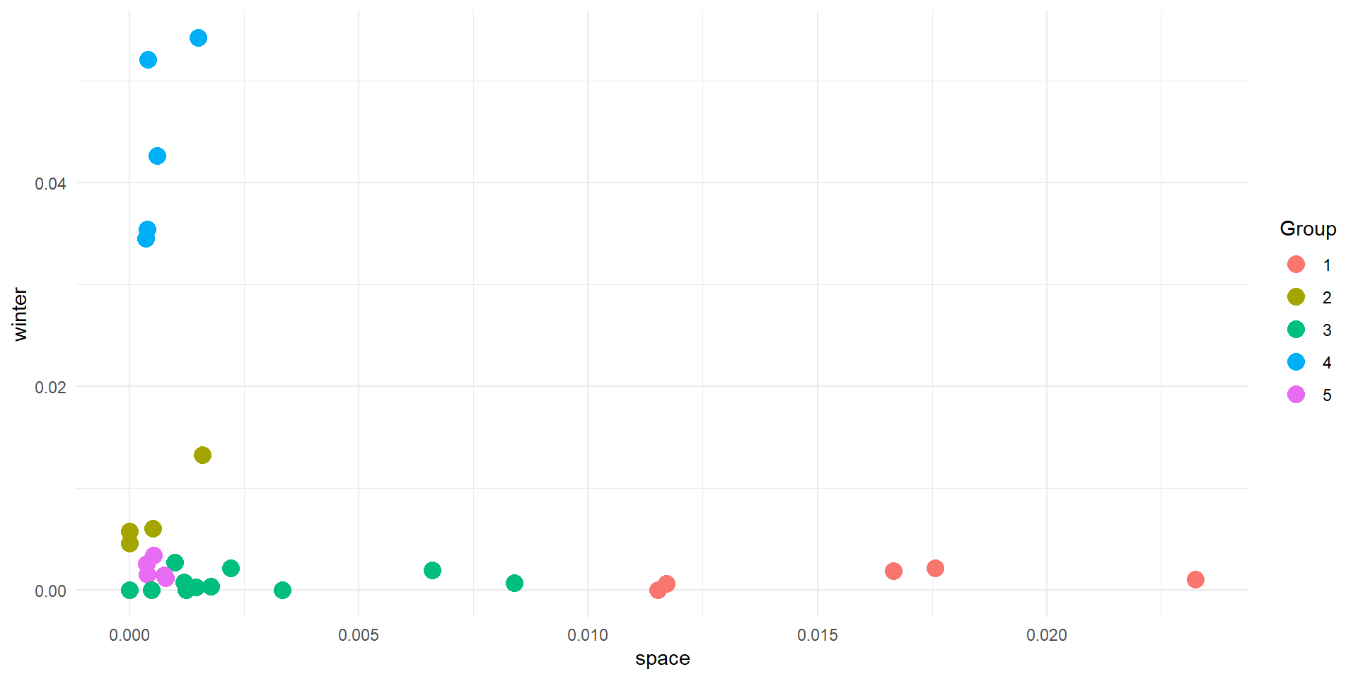
Interpreting
- The algorithm knows nothing about your data, except how close points are in space
- You need to use your knowledge to interpret the results